What is Regression?
Regression is a technique in where it is aimed to estimate the value of a a dependent variable, \(y\), and a predictor variable, \(x\). The most common method in which this is performed is by Ordinary Least Squares (OLS) which reduces the residual variance. This is a method that is used when there is a linear relationship between the predictor and the dependent variable. In linear regression the expected value of Y is the population mean for a particular value of x, this can be expressed as: \(E(Y|X = x) = \alpha + \beta X \), where \(\alpha\), also known as \({\beta_{0}}\), is the value that \(Y\) takes when \(X\) is 0. \(\beta\) is unit increase of \(Y\) for each value of \(X\).
Regression is similar to correlation, in that it is a measure of the association
between variables. However where as correlation, \(\rho\), is a measure of the covariance, \(E[(X - \mu_{x})(Y - \mu_{y})]\), between two variables, regression is the estimation of
one variable conditional on one or more predictor variables.
Below is an example of the different correlation values that can occur, \(\rho\) is between -1 and 1 where both -1 and 1 are perfect correlation between the
two variables.
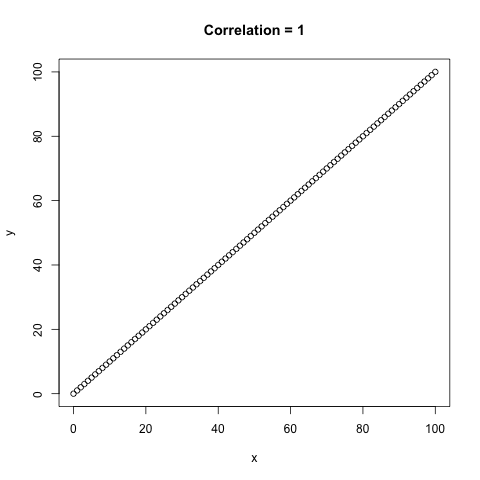
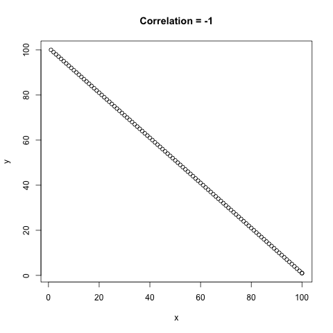
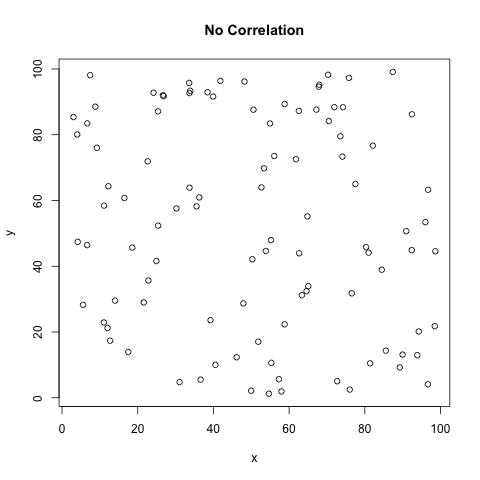 Figure 1 - A comparison of the different types of correlation, \(\rho\).
As you can see correlation is very similar to a regression, however there are not the same. Correlation of two variables will be the same regardless of which one is defined as x and y, as \(\rho = \frac{Cov(X,Y)}{SD(X)SD(Y)}\). Whereas with regression the outcome variable is conditional on the predictor variable(s) so \(Y|X\) is different to \(X|Y\). This can be shown algebraically with the regression coefficient, \(\hat{\beta}\).
For \(X|Y\):\({\hat{\beta}}_{X|Y} = \frac{S_{xy}}{{{SD}_{y}}^{2}}\)
It turns out that the coefficient of Y|X and X|Y multiplied together will provide the estimate of the correlation coefficient. Therefore the correlation coefficient \(\rho\) will not be equal to the regression coefficient. The only exception is when the correlation coefficient is equal to 1 or -1 i.e. perfect correlation.
In the next section the methods of regression will be explored using a simple example where there exists only one predictor (\(X\)) variable and one outcome variable (\(Y\)). However this can be used in more complex situations, in which the principles remain the same.
This is assuming that the outcome is univariable, see below for meaning, and that the assumptions for linear regression are met.
The assumptions for linear regression are:
The sum of squares is an estimate of the the squared distance of a given point from it's mean and is used to estimate the coeficients used in regression. It is also often referred to as the deviation of a given point from the mean, summed over all observations. When there is no fitted regression model the residual sum of squares is actually equivalent to the total sum of squares.
\[{SS}_{total} = {SS}_{res(null)} = \sum_{i=1}^{n}(y_{i} - \bar{y})^{2}\]
The OLS method aims to reduce the residual sum of squares by fitting the regression model between the points. A fitted regression line will generate predicted values,
\({\hat{y}}_{i}\). In the OLS method of regression the total sum of squares under the alternate is partitioned to the regression sum of squares, and the alternate residual sum of squares:
\[{SS}_{total} = {SS}_{res(alt)} + {SS}_{reg}\]
\[\sum_{i=1}^{n}(y_{i} - \bar{y})^{2} = \sum_{i=1}^{n}(y_{i} - {\hat{y}}_{i})^{2} + \sum_{i=1}^{n}({\hat{y}}_{i} - \bar{y})^{2}\]
This is actually known as the analysis of variance (ANOVA) and is used to try and explain the variance of the outcome variable given a list of predictors, which in this case is just one. So now the residual sum of squares is the sum over the distance between the predicted values \({\hat{y}}_{i}\) and the observed values \(y\).
In the regression model the fitted values can be defined as \({\hat{y}}_{i} = \hat{\alpha} + {\hat{\beta}}x_{i}\), where \(\hat{\alpha}\) and \(\hat{\beta}\) are maximum likelihood estimates. So the residuals can actually be rewritten as:
\[{SS}_{res(alt)} = \sum_{i=1}^{n}(y_{i} - \hat{\alpha} - \hat{\beta}x_{i})^{2}\]
Where:
The Simple Linear Regression Model
In the case of linear regression it turns out that the variance follows an F distribution so when in this model, with only one predictor, the F test statistic can be used to determine if the variance in Y is better explained when X is a predictor, compared to when there is no predictor in the model.
\[F = \frac{{SS}_{Reg}/p}{{SS}_{Res(Alt)}/(n-(p+1))}\] Where:- \(p\) is the degrees of freedom, which is the number of predictor variables, in this case there is only 1
- \(n-(p+1)\) is the degrees of freedom of the residuals, where \(n\) is the sample size and \((p+1)\) is the number of paramters including the constant
Terminology
| Univariable: | One single predictor variable | Univariate: | One single outcome variabe |
| Multivariable: | More than one predictor variable | Multivariate: | More than one outcome variable |
| Sum of Squares: | Sum of the deviation squared of individual points from the mean, e.g. for X, \(SS_{xx} = \sum_{i=1}^{n}(x_{i} - \bar{x})^{2}\) | Sum of Cross Product | Sum of the deviation of the outcome variable, y, and the preictor variable x, \(SS_{xy} = \sum_{i=1}^{n}(y_{i} - \bar{y})(x_{i} - \bar{x})\) |
| Variance Estimator: | As the MLE estimate of the Variance is biased towards the estimated line the following estimator is used instead; \({\hat{\sigma}}^2 = \sum_{i=1}^{n} {\hat{\varepsilon}}^{2} = \sum_{i=1}^{n}\frac{(y_{i} - {\hat{\alpha}} - {\hat{\beta}}x_{i})^{2}}{n-2}\) | Test | Test |
Back to Top